Finding The Shortest Path Between Two Points On A Graph Using Dijkstra’s Algorithm

Have you ever wondered how maps work and how they are able to show you the fastest route to your destination? Prior to becoming a software engineer, the idea of how navigation works was quite elusive. In this article, I will shed some light on Dijkstra’s algorithm and attempt to briefly explain how it can be used to calculate the shortest path between any two points.

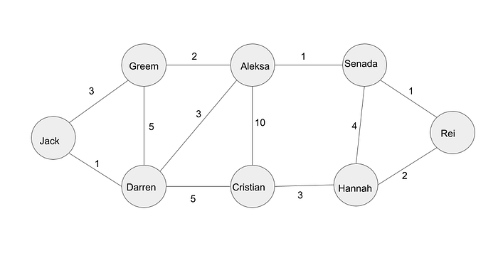
Before we delve into the code of the algorithm, let’s make sure that we are comfortable working with the Tree data structure. A Tree data structure is used to structure and organize data points that have a hierarchal relationship between them. The following diagram is an example of a Tree data structure:

Each circle above denotes a data point that we call “node”. The nodes are connected to one another through a branch that we call “edge”. The values alongside the edges are called “weights”. These weights determine the price, cost, or efficiency to go from one node to the next. A higher number indicates a less efficient route. For example, looking at the Tree structure above, we can see that going from “Jack” to “Darren” is much cheaper than going from “Jack” to “Greem.”

Having edges with weights is an example of a weighted graph/tree. This is useful info to add to a Tree data structure because, in a real-world scenario, you want highway roads to have less weight than local street roads.

Now that you have an understanding of what a Tree data structure is, let’s dedicate the rest of the article to answering the following question:

What is the fastest way to get from “Jack” to “Rei”?

Well, there are so many different routes that we can take to get from “Jack” to “Rei”. We will have to calculate the distances from every possible combination of nodes and then choose the shortest. For example, we can follow this route: “Jack” >“Darren” > “Cristian” > “Hannah” > “Rei”. If we calculate the distance between them (adding up the weights between the nodes) this will give us a total distance or cost of 11. But an alternative way would be, “Jack” >“Greem” > “Aleksa” > “Senada” > “Rei”, which will yield a total distance or cost of 7. So this route with the cost of 7 is way more efficient than the previous route with a cost of 11.

But there are routes that could be more efficient than 7 and 11. For example, if we take the path “Jack” >“Darren” > “Aleksa” > “Senada” > “Rei” this will give us a cost of 6, which is more efficient than the previous two paths we took.

I think you get the point now! You can manually traverse the tree above and search for the shortest path, but you may be wondering how are we going to do that if we have thousands or even millions of nodes? This is where the power of Dijkstra’s algorithm comes into play.

Dijkstra’s Algorithm

Below are the fundamental steps that are taken by the Dijkstra’s algorithm to find the shortest path between two nodes:

1. Find the start node and initialize its cost/distance to zero and set the cost/distance of all other nodes to infinity. We will call this the cost object. We will also initialize an empty array which we’ll call visited to keep track of nodes that we have analyzed. We will also need to keep track of the parent of each node so that we can track the shortest path taken. We’ll call this parentNodes.
2. calculate the cost/distance between the start node and its children, updating the cost object of the child node with the new value if it’s lower. Alongside updating the cost object, we will update the parentNodes of this child node.
3. Add the analyzed node to the visited array.
4. Analyze the next lowest node (we can get that from the cost object) in a similar fashion to step 2. Repeat steps 2–4 until all nodes have been visited.
5. Now we can determine the fastest path by examining the parentNodes object and trace the path from the finish node to the start node.

Implementation

To remind ourselves, this is our tree that we discussed above:

Let us convert our Tree data structure shown above to JSON so we can traverse the nodes.

in our graph object above, each node in our Tree is used as a key and its values are its neighbors with their associated weight.

We need to initialize a “cost” variable to keep track of the lowest cost nodes. We initialize the cost of the starting node to zero and all other nodes to infinity:

Please note that instead of the “cost” object above, we could have used a priority queue to keep track of our lowest cost nodes traversal. Instead of using a priority queue, I will be implementing a helper method that will retrieve the lowest cost node. The method can be implemented as follow:

After we initialized our “cost” object, we need a way to keep track of the parents of each node in our cost object so that we can retrieve the shortest paths. Initially, it will only contain the last node and the children of the starting node. We’ll also initialize a “visited” array to keep track of nodes that we already visited so that we don’t unnecessarily analyze a node multiple times.

Now that we have our housekeeping variables setup, we can kick off the algorithm. We will iterate through each node and if the node has been analyzed? if so, skip to the next node. If it hasn’t been analyzed then do the following:

1. calculate the distance from the start node to each of its neighbors, if the neighbor’s calculated cost is lower than what’s in the costs array, replace the value in the “costs” array with the new value. Also, point the parent of the child in the “parentNodes” to the current node being analyzed.
2. After analyzing or neighboring nodes, add the current node to the “visited” array so we don’t analyze it again. Then find the closest child node that hasn’t been analyzed and repeat step 1 again until all nodes have been visited.

The code for the above steps is as follows:

After we finish analyzing all nodes we can simply look at our “parentNodes” object and back-trace from the finish node all the way to the start node. This can be done like so:

In the above code, we are generating the sequence of nodes from the end to the start, so if we simply reverse that list, we’ll have the path from the start node(“Jack”) to the end node (“Rei”).

The complete code along with a demo application can be found here.